100倍更快 — 让您的RAG应用支持数十亿个嵌入
在并行计算中计算余弦相似度
在 RAG 应用程序中最大的问题之一是它们的计算检索时间。想象一下,你有一个含有一万亿条嵌入向量记录的向量数据库。当你尝试将用户查询与一万亿个向量进行匹配时,肯定需要超过一分钟来获取正确的信息。
我们能否通过在CPU核心上使用并行处理来将获取正确信息的时间减少到秒级别?
减少时间包括寻找计算用户查询嵌入向量与存储在您的向量数据库中的百万、十亿甚至万亿个其他嵌入向量之间余弦相似度的高效方法。
Chunkdot是根据MIT许可证特别设计用于此目的的工具,提供了针对密集和稀疏矩阵的多线程矩阵乘法。它适用于通过分割项目矩阵表示(嵌入)并使用Numba加速计算来计算大量项目的K个最相似项。
Chunkdot的GitHub存储库
有许多可在HuggingFace上获得的数据集,提供了超过一百万条记录的嵌入向量,比如来自Qdrant的这个数据集。您可以使用它来测试Chunkdot的性能。然而,为了进行详细的性能测量,我们将使用NumPy库生成不同维度的随机嵌入向量。
我们将比较两种方法,一种来自Chunkdot,第二种是余弦相似度的伪代码。我们将观察性能如何受到尺寸和维度增加的影响。我将使用Kaggle(无GPU)笔记本来完成这个任务,以确保结果的一致性。
此博客的所有代码均可在我的GitHub代码库中找到。
目录
- 设置舞台
- 编码 伪代码算法
- 编码Chunkdot算法
- 编码计算时间函数
- 测试10K向量嵌入
- 测试100k个矢量嵌入
- 测试1百万个向量嵌入
- 可视化可扩展性影响
- Chunkdot的特点
- 下一步是什么
搭建舞台
Chunkdot 需要与其他库相似的安装过程。
# installing chunkdot
pip install chunkdot
在运行任何东西之前,我们必须首先检查我们Kaggle环境中可用的内存。
# Checking available memory
!free -h
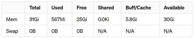
检查可用的内存对于Chunkdot来说非常重要。随着向量数据库的大小增加,计算内存也会增加。为了防止超出可用内存,监视硬件中剩余的内存非常重要。在我的情况下,除了 Buff/Cache 外,可用空间为25GB。
让我们导入必要的库。
# to matrix generate matrices
import numpy as np

# importing cosine similarity module from chunkdot
from chunkdot import cosine_similarity_top_k

# to calculate computation time
import timeit
编程 伪代码 算法
我们将首先构建一个伪代码算法,用于计算用户查询向量与可能存储在数据库或本地的其他数百万个向量之间的余弦相似度。
def cosine_pseudocode(query_v, doc_v, num_indices):
    """
    Retrieve indices of the highest cosine similarity values between
    the query vector and embeddings.

    Parameters:
        query_v (numpy.ndarray): Query vector.
        doc_v (list of numpy.ndarray): List of embedding vectors.
        num_indices (int): Number of Top indices to retrieve.

    Returns:
        list of int: Indices of the highest cosine similarity values.
    """
    cosine_similarities = []  # Initialize an empty list to store cosine similarities

    query_norm = np.linalg.norm(query_v)  # Calculate the norm of the query vector

    # Iterate over each documents embedding vectors in the list
    for vec in doc_v:
        dot_product = np.dot(vec, query_v.T)  # Calculate dot product between embedding vector and query vector
        embedding_norm = np.linalg.norm(vec)  # Calculate the norm of the embedding vector
        cosine_similarity = dot_product / (embedding_norm * query_norm)  # Calculate cosine similarity
        cosine_similarities.append(cosine_similarity)  # Append cosine similarity to the list

    cosine_similarities = np.array(cosine_similarities)  # Convert the list to a numpy array

    # Sort the array in descending order
    sorted_array = sorted(range(len(cosine_similarities)), key=lambda i: cosine_similarities[i], reverse=True)

    # Get indices of the top two values
    top_indices = sorted_array[:num_indices]

    # Return the indices of highest cosine similarity values
    return top_indices
这个余弦相似度函数与任何库无关,除了NumPy之外,它需要三个输入:
- 查询_v 用户查询的嵌入向量
- 文档的嵌入向量被存储在某个地方。
- num_indices 从文档中提取相似的前k个结果的索引编号
编码Chunkdot算法
现在我们已经编写了伪代码算法,下一步是编写Chunkdot余弦相似度函数。
def cosine_chunkdot(query_v, doc_v, num_indices, max_memory):
    """
    Calculate cosine similarity using the chunkdot library.

    Parameters:
        query_v (numpy.ndarray): Query vector.
        doc_v (numpy.ndarray): List of Embedding vectors.
        num_indices (int): Number of top indices to retrieve.
        max_memory (float): Maximum memory to use.

    Returns:
        numpy.ndarray: Top k indices.
    """

    # Calculate Cosine Similarity
    cosine_array = cosine_similarity_top_k(embeddings=query_v, embeddings_right=doc_v,
                                          top_k=num_indices, max_memory=max_memory)  # Calculate cosine similarity using chunkdot

    # Get indices of the top values
    top_indices = cosine_array.nonzero()[1]

    # return the top similar results
    return top_indices
这个Chunkdot函数接受四个输入:
- 查询_v用户查询的嵌入向量
- doc_v 存储在某处的文档嵌入向量
- num_indices 相似的前 top_k 结果的文档索引号
- max_memory表示您用于计算的可用内存,其值以字节表示。例如,1E9表示1GB,10E9表示10GB,依此类推。
让我们在一个样本数据集上测试我们的两个功能,观察它们的输出结果。
doc_embeddings = np.random.randn(10, 100) # 10 document embeddings (100 dim)

user_query = np.random.rand(1,100) # 1 user query (100 dim)

top_indices = 1 # number of top indices to retrieve

max_memory = 5E9 # maximum memory to use (5GB)

# retrieve indices of the highest cosine similarity values using pseudocode
print("top indices using pseudocode:", cosine_pseudocode(user_query, doc_embeddings, top_indices))

# retrieve indices of the highest cosine similarity values using chunkdot
print("top indices using chunkdot:", cosine_chunkdot(user_query, doc_embeddings, top_indices, max_memory))
### OUTPUT ###
top indices using pseudocode: [4]
top indices using chunkdot: [4]
### OUTPUT ###
我生成了10个文档嵌入向量的随机嵌入向量,每个维度都是100,并且一个用户查询是一个具有相同维度的单一嵌入向量。top_indices参数设置为1,表示根据最高的余弦相似度,它将返回来自文档嵌入的只有一个相似项的索引。内存使用量已设置为5E9,相当于5GB。我们的两个函数都返回相同的索引4,表明我们准确编码了这两个函数。
编码计算时间函数
我们还需要创建一个计时函数,用于测量这两个函数所需的计算时间并输出结果。
# calculate time taken
def calculate_execution_time(query_v, doc_v, num_indices, max_memory, times):

    # calculate time taken to execute the pseudocode function
    pseudocode_time = round(timeit.timeit(lambda: cosine_pseudocode(query_v, doc_v, num_indices), number=times), 5)

    # calculate time taken to execute the chunkdot function
    chunkdot_time = round(timeit.timeit(lambda: cosine_chunkdot(query_v, doc_v, num_indices, max_memory), number=times), 5)

    # print the time taken
    print("Time taken for pseudocode function:", pseudocode_time, "seconds")
    print("Time taken for chunkdot function:", chunkdot_time, "seconds")
我们已经回顾了传递到此函数的参数。这里唯一的新参数是times,它告诉函数您想要运行代码的次数。让我们在更大的规模上测试Chunkdot的性能效率。
测试10k矢量嵌入
我们将从一个合理的文件嵌入数量开始,10000个,这与一个小规模的领域特定RAG应用相当。我将每个嵌入向量的维度设置为1536,这相当于OpenAI嵌入模型text-embedding-3-small。
让我们通过运行它们100次来计算每种方法的计算时间。
doc_embeddings = np.random.randn(10000, 1536) # 10K document embeddings (1536 dim)

user_query = np.random.rand(1,1536) # user query (1536 dim)

top_indices = 1 # number of top indices to retrieve

max_memory = 5E9 # maximum memory set to 5GB

# compute the time taken to execute the functions
calculate_execution_time(user_query, doc_embeddings, top_indices, max_memory, 100)
对于10k个文档嵌入,维度为1536,运行两个算法100次,以下是比较结果:
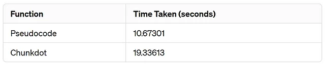
Chunkdot花费比我们的伪代码更多的时间。这是因为它首先创建块并在每个块上执行计算,然后再合并它们。因此,对于这个小规模的例子来说,它可能不是一个合适的解决方案。然而,当我们在后面处理一个更大的例子时,您将看到Chunkdot的好处。
测试100k个向量嵌入
对于10K,我们的伪代码方法取胜,但现在让我们将我们的文档嵌入向量增加到100K个向量,这与中等规模的RAG应用程序相当。
让我们计算每种方法的计算时间,但这次我们将times参数设置为1(只运行一次代码),因为向量的数量很大,没有必要多次进行计算。
doc_embeddings = np.random.randn(100000, 1536) # 100K document embeddings (1536 dim)

user_query = np.random.rand(1,1536) # user query (1536 dim)

top_indices = 1 # number of top indices to retrieve

max_memory = 5E9 # maximum memory set to 5GB

times = 1 # number of times to execute the functions

# compute the time taken to execute the functions
calculate_execution_time(user_query, doc_embeddings, top_indices, max_memory, times)
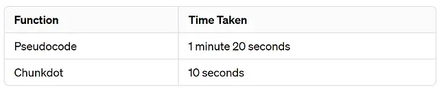
对于100k个文档嵌入,维度为1536,运行两个算法一次,这是比较结果:
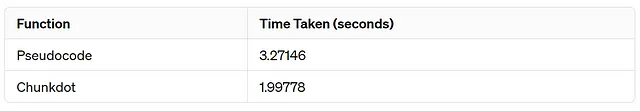
Chunkdot相比我们的伪代码使用时间更少,几乎只有一半。现在我们看到了Chunkdot的很有前景的影响。
测试100万个向量嵌入
在处理涉及数百万嵌入的任务时,你需要首先检查文档嵌入向量占用多少内存。
# 1 Million document embeddings (1536 dim)
doc_embeddings = np.random.randn(1000000, 1536)

# user query (1536 dim)
user_query = np.random.rand(1,1536)

# Check the memory size of doc_embeddings and user_query embedding
print(doc_embeddings.nbytes / (1024 * 1024 * 1024),
      user_query.nbytes / (1024 * 1024))
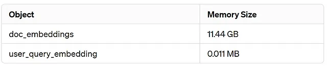
我们的文档嵌入大约占用12GB的空间。让我们检查剩余可用空间。
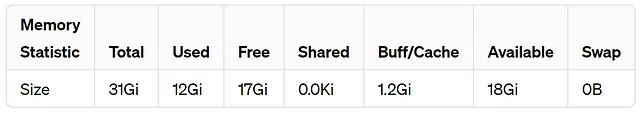
我们有最高可用的17GB内存。为了避免任何内存错误,我们将为max_memory参数设置一个安全值,即12GB。让我们看看结果。
# 1 Million document embeddings (1536 dim)
doc_embeddings = np.random.randn(1000000, 1536)

# user query (1536 dim)
user_query = np.random.rand(1,1536)

top_indices = 1 # number of top indices to retrieve

max_memory = 12E9 # maximum memory set to  --- 12GB ---

times = 1 # number of times to execute the functions

# compute the time taken to execute the functions
calculate_execution_time(user_query, doc_embeddings, top_indices, max_memory, times)
ChunkDot确实有效地减少计算量。当您打算构建一个成熟的RAG应用时,您应该考虑从至少一百万个查询开始。使用高维度的嵌入模型,最多达到4000个。这种方法将变得更加高效。
可视化可扩展性影响
让我们可视化地看一下将文档嵌入向量的数量从10,000增加到非常大的数值所带来的影响。
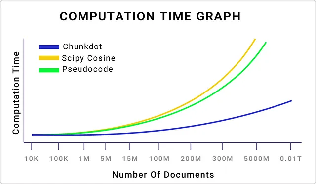
我绘制了三种方法,而Chunkdot是基于增加文档嵌入数量最优的方法。现在,让我们来看看嵌入向量的维度如何影响计算时间。
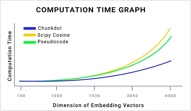
我在增加向量维度时使用了10万个文档,观察到与增加文档数量时相同的行为。
Chunkdot的特点
Chunkdot 有一个功能,可以显示一个进度条,帮助您跟踪剩余计算量。
doc_embeddings = np.random.randn(100000, 1536) # 100K document embeddings (1536 dim)

user_query = np.random.rand(1,1536) # user query (1536 dim)

top_indices = 100 # number of top indices to retrieve

max_memory = 5E9 # maximum memory set to 5GB

# with progress bar
output_array = cosine_similarity_top_k(user_query, doc_embeddings,
                        top_k=top_indices,
                        show_progress=True)
Chunkdot的输出是一个稀疏矩阵,你可以使用以下方法将其转换为数组:
# converting the ouput
output_array.toarray()
您可以使用Chunkdot仅进行文档嵌入,该方法将为每个文档嵌入元素返回前k个最相似的元素。
# total 5 documents embeddings
embeddings = np.random.randn(5, 256)

# return top 2 most similar item index for each
cosine_similarity_top_k(embeddings, top_k=2).toarray()
### OUTPUT ###
array([[1.        , 0.        , 0.        , 0.        , 0.09924064],
       [0.        , 1.        , 0.        , 0.09935381, 0.        ],
       [0.02358785, 0.        , 1.        , 0.        , 0.        ],
       [0.        , 0.09935381, 0.        , 1.        , 0.        ],
       [0.09924064, 0.        , 0.        , 0.        , 1.        ]])
### OUTPUT ###
同样,您可以通过将top_k参数设置为负值来返回最不相似的前几个项目。
# total 5 documents embeddings
embeddings = np.random.randn(5, 256)

# return top 2 most dissimilar item index for each
# Top_K = -2
cosine_similarity_top_k(embeddings, top_k=-2).toarray()
### OUTPUT ###
array([[ 0.        ,  0.        , -0.04357524,  0.        , -0.05118288],
       [ 0.        ,  0.        ,  0.        ,  0.01619543, -0.01836534],
       [-0.04357524,  0.        ,  0.        , -0.02466613,  0.        ],
       [ 0.        ,  0.01619543, -0.02466613,  0.        ,  0.        ],
       [-0.05118288, -0.01836534,  0.        ,  0.        ,  0.        ]])
### OUTPUT ###
这可能不适用于您的情况,但是如果您处理的稀疏嵌入维度高达10K,您可以使用密度参数更高效地减少计算。
# for creating sparse embeddings
from scipy import sparse

# creating spare matrix with 100K documents (10K dim each)
# defining density of 0.005
embeddings = sparse.rand(100000, 10000, density=0.005)

# using all you system's memory
cosine_similarity_top_k(embeddings, top_k=50)
接下来是什么
如果你想了解Chunkdot算法的工作原理,请查看作者的这篇令人惊叹的博客。Chunkdot的最大优点之一是它可以在CPU核心上运行。在将来,他们计划整合GPU支持,这将极大地减少计算时间。如果你的本地环境没有足够的RAM,你可以使用像Kaggle或GitHub Codespaces这样的平台,云CPU核心和RAM的成本非常低,与GPU成本相比。别忘了检查官方的GitHub存储库以及他们的博客,因为它非常详细地解释了Chunkdot的工作原理。